Sigolyori’s Blog - 회귀 모델에서 계수 p-value의 의미

회귀를 통한 데이터 분석을 수행하면, 계수값과 아울러 계수 값의 p-value도 확인할 수 있습니다.

계수값의 p-value는 어떤 의미를 가지고 있는지 알아보겠습니다.

데이터는 kaggle에 올라와 있는 autompg 데이터셋을 사용했습니다.

import pandas as pd

df = pd.read_csv('../../autompg-dataset/auto-mpg.csv')

df.head()

	mpg	cylinders	displacement	horsepower	weight	acceleration	model year	origin	car name
0	18.0	8	307.0	130	3504	12.0	70	1	chevrolet chevelle malibu
1	15.0	8	350.0	165	3693	11.5	70	1	buick skylark 320
2	18.0	8	318.0	150	3436	11.0	70	1	plymouth satellite
3	16.0	8	304.0	150	3433	12.0	70	1	amc rebel sst
4	17.0	8	302.0	140	3449	10.5	70	1	ford torino

acceleration에 따른 mpg를 회귀 분석 수행한다고 가정하겠습니다.

indep = 'acceleration'
dep = 'mpg'

scikit-learn의 LinearRegression을 통해 선형 회귀 분석을 할 수 있습니다.

from sklearn.linear_model import LinearRegression

lr = LinearRegression()

# 독립변수 에러로 인해 reshape(-1,1)을 추가하여 주었습니다.
model = lr.fit(df[indep].values.reshape(-1,1), df[dep])

# 변수 계수
model.coef_

array([1.19120453])

# 절편 계수
model.intercept_

4.969793004253901

선형 회귀를 수행하고, 변수 및 절편의 계수를 확인할 수 있었습니다.

위와 같이 전체에서 선형 회귀를 진행하는 것이 아니라, 일부 샘플을 추출한 다음 선형 회귀식을 만들어 계수를 여러 번 뽑을 수도 있겠습니다.

이를 통해 계수값의 변동성을 아는 것이 목표이자, 동시에 p-value의 기능입니다.

from sklearn.utils import resample

반복을 위한 함수를 boot라는 이름으로 정의합니다.

def boot():
    idx = resample(range(len(df)), replace=False, n_samples=100)
    lr = LinearRegression()
    model = lr.fit(df.iloc[idx][indep].values.reshape(-1,1), df.iloc[idx][dep])
    return model.coef_[0]

values = [boot() for i in range(1000)]

import numpy as np

# 95% 신뢰구간의 하한
lp = np.quantile(values, q=0.025); lp

0.7308445555728666

# 95% 신뢰구간의 상한
hp = np.quantile(values, q=0.975); hp

1.6430318330598581

# 계수의 값
model.coef_

array([1.19120453])

import matplotlib.pyplot as plt

plt.hist(values)
plt.axvline(x=lp, ls=':')
plt.axvline(x=hp, ls=':')
plt.title('반복추출된 계수표본(model.coef_)의 분포')

Text(0.5, 1.0, '반복추출된 계수표본(model.coef_)의 분포')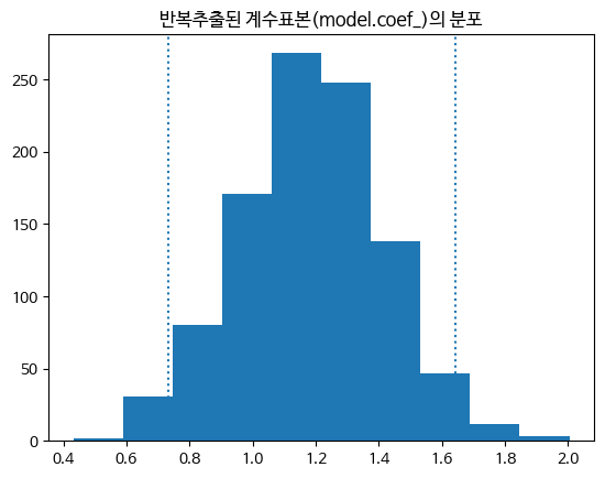

위 결과를 statsmodels로 수행한 p-value 및 신뢰구간과 비교하겠습니다.

import statsmodels.api as sm

model = sm.OLS(df[dep], df[indep])

results = model.fit()

results.summary()

OLS Regression Results
Dep. Variable:	mpg	R-squared (uncentered):	0.917
Model:	OLS	Adj. R-squared (uncentered):	0.917
Method:	Least Squares	F-statistic:	4389.
Date:	Thu, 19 Jan 2023	Prob (F-statistic):	1.02e-216
Time:	06:02:43	Log-Likelihood:	-1346.9
No. Observations:	398	AIC:	2696.
Df Residuals:	397	BIC:	2700.
Df Model:	1
Covariance Type:	nonrobust

	coef	std err	t	P>\|t\|	[0.025	0.975]
acceleration	1.5007	0.023	66.249	0.000	1.456	1.545

Omnibus:	11.929	Durbin-Watson:	0.760
Prob(Omnibus):	0.003	Jarque-Bera (JB):	12.496
Skew:	0.421	Prob(JB):	0.00193
Kurtosis:	2.788	Cond. No.	1.00

Notes:
[1] R² is computed without centering (uncentered) since the model does not contain a constant.
[2] Standard Errors assume that the covariance matrix of the errors is correctly specified.

주목해야 할 부분은 coef, P>|t|, 0.025(95% 신뢰구간 하한), 0.975(95% 신뢰구간 상한)입니다.

재표본추출(부트스트랩)을 통해 얻은 결과와 큰 차이가 없음을 알 수 있습니다. 표본통계량의 변동성을 확인할 때는 재표본추출을 사용할 수 있음을 알 수 있습니다.