library(tidyverse)
library(survival)고객 이탈 예측을 위한 생존분석
⭐
고객 이탈 예측에 Kaplan-Meier 생존분석과 Cox 비례위험모형을 적용하는 방법을 R로 구현합니다.
탐구 동기 및 목표
- 강의 시간에는 의학 분야 예제로 생존분석을 공부했는데, 기존에 관심있던 마케팅 분야에서 생존분석이 어떻게 활용될 수 있는지 탐구하고자 함.
- 고객 데이터의 생존함수와 위험함수로부터 데이터에 대한 이해를 넓히고자 하며, 이후 Cox 비례 위험 모형을 적합한 후 모형의 예측 정도를 확인하고자 함.
data("churn_tel", package = "liver")
# Check actual column names - may differ from documentation
names(churn_tel)
[1] "customer_ID" "gender" "senior_citizen"
[4] "partner" "dependent" "tenure"
[7] "phone_service" "multiple_lines" "internet_service"
[10] "online_security" "online_backup" "device_protection"
[13] "tech_support" "streaming_TV" "streaming_movie"
[16] "contract" "paperless_bill" "payment_method"
[19] "monthly_charge" "total_charge" "churn" 데이터 설명
liver 패키지의 churn_tel 데이터에는 7,043개의 관측치에 대한 21개 변수가 존재함(Mohammadi and Burke 2023).
| 변수 | 설명 |
|---|---|
| customer.ID | Customer ID. |
| gender | Whether the customer is a male or a female. |
| senior.citizen | Whether the customer is a senior citizen or not (1, 0). |
| partner | Whether the customer has a partner or not (yes, no). |
| dependent | Whether the customer has dependents or not (yes, no). |
| tenure | Number of months the customer has stayed with the company. |
| phone.service | Whether the customer has a phone service or not (yes, no). |
| multiple.lines | Whether the customer has multiple lines or not (yes, no, no phone service). |
| internet.service | Customer’s internet service provider (DSL, fiber optic, no). |
| online.security | Whether the customer has online security or not (yes, no, no internet service). |
| online.backup | Whether the customer has online backup or not (yes, no, no internet service). |
| device.protection | Whether the customer has device protection or not (yes, no, no internet service). |
| tech.support | Whether the customer has tech support or not (yes, no, no internet service). |
| streaming.TV | Whether the customer has streaming TV or not (yes, no, no internet service). |
| streaming.movie | Whether the customer has streaming movies or not (yes, no, no internet service). |
| contract | The contract term of the customer (month to month, 1 year, 2 year). |
| paperless.bill | Whether the customer has paperless billing or not (yes, no). |
| payment.method | The customer’s payment method (electronic check, mail check, bank transfer, credit card). |
| monthly.charge | The amount charged to the customer monthly. |
| total.charges | The total amount charged to the customer. |
| churn | Whether the customer churned or not (yes or no). |
문제에서 관심있는 event인 churn은 고객에 대해서 한 번만 발생하는 event로, 그 값은 yes 또는 no 임.
비모수적 생존함수 추정 (카플란-마이어 방법)
데이터로부터 생존곡선을 산출하는 Kaplan-Meier 방법을 적용함.
만약 관측치가 censored 된 경우는 0, 그렇지 않으면 1로 status indicator를 정의함. 예제에서 censored 되는 경우는 실험이 종료될 때까지 event가 발생하지 않은 경우로, 다른 censoring의 경우인 loss to follow-up은 해당 데이터에서 발생하지 않음.
time <- churn_tel$tenure
status <- ifelse(churn_tel$churn == "yes", 1, 0)

surv.fit <- survfit(Surv(time, status) ~ 1)

plot(surv.fit, main="카플란-마이어 생존함수 추정",
     xlab="tenure", ylab="survival")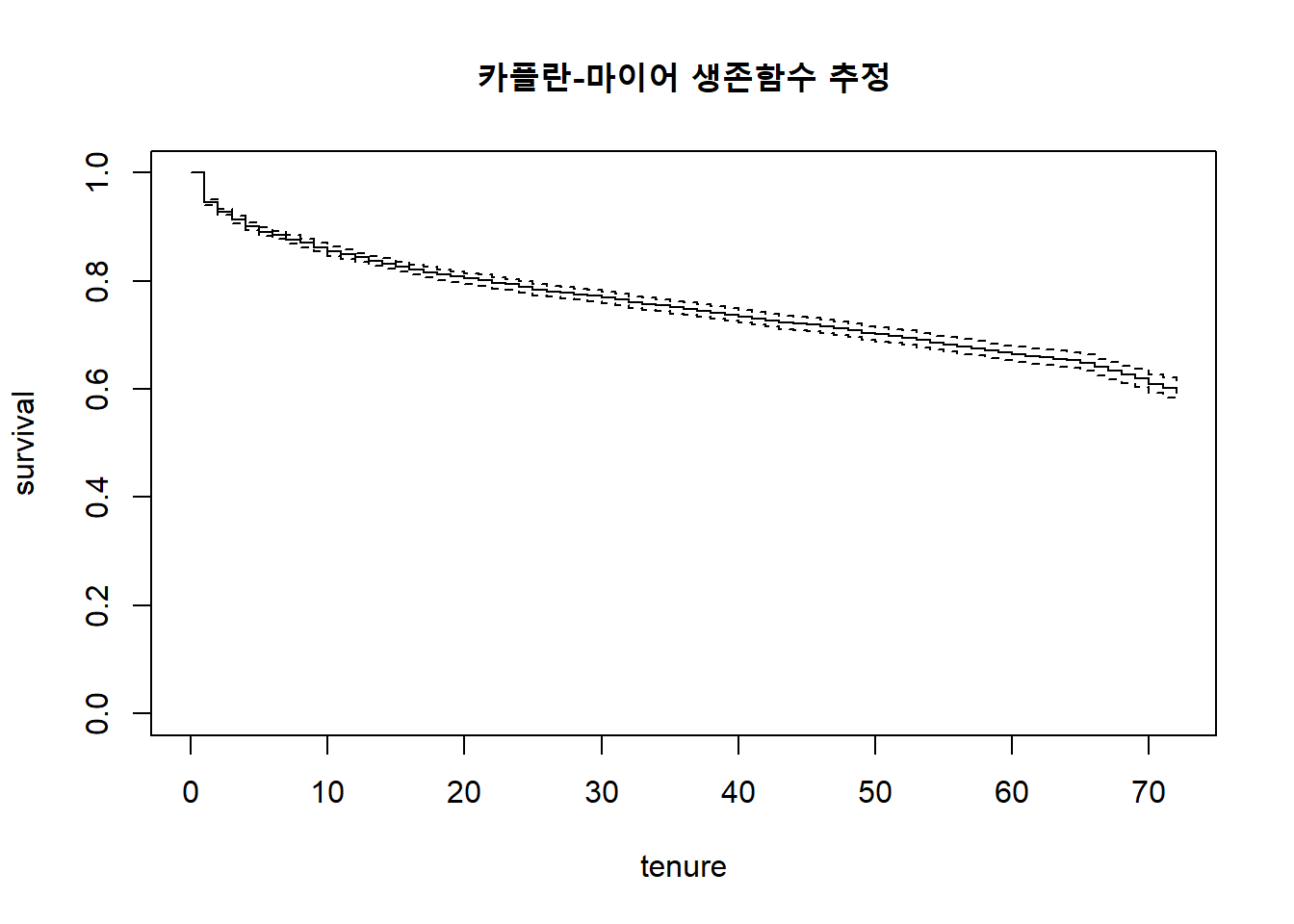
output <- tibble(time=surv.fit$time,
                 surv=surv.fit$surv) %>%
  mutate(space=time*surv) %>%
  summarise(avg_life_time=mean(space)) %>%
  pull()


print(output)
[1] 25.68115생존함수에서 구한 평균이 실제 구독 기간의 평균을 의미하는 것은 아님. 하지만 해당 추정치는 고객 유지 예산 예산 배정의 문제에 도움을 줄 수 있음(Linoff and Berry 2011).
surv.fit <- survfit(Surv(time, status) ~ internet_service,
                    data=churn_tel)
Hazard의 경향 확인
time \(t\)에 대한 Hazard는 \[\frac {\text{The number of events at time t}} {\text{population at risk at time t}} \]
Kaplan-Meier 적합 시 생성되는 table을 활용하여 데이터로부터 경험적 Hazard ratio를 구할 수 있음.
구독 모델의 경우 초기 진입 이후 프로모션이 끝나면 이탈하는 고객이 있음으로 시간에 따른 Hazard의 모양은 U-자형으로 보임.
tibble(time=surv.fit$time,
       n.event=surv.fit$n.event,
       n.risk=surv.fit$n.risk) %>%
  mutate(hazard.ratio=n.event/n.risk) %>%
  ggplot() +
  geom_line(aes(x=time, y=hazard.ratio)) +
  ggtitle("72주 기간 동안 hazard ratio의 경향")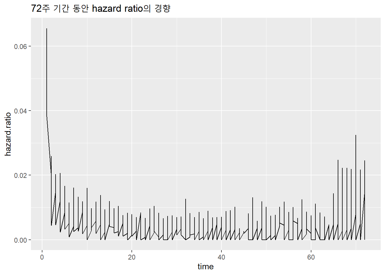
Cox 비례 위험 모형
idx <- churn_tel %>%
  mutate(idx = row_number()) %>%
  filter(internet_service != "No") %>%
  filter(phone_service != "No") %>%
  pull(idx)
data <- churn_tel[idx, ] %>%
mutate(across(where(is.factor), droplevels)) %>%
select(-c(customer_ID, phone_service, total_charge))N <- nrow(data) * 0.2
test <- sample(nrow(data), N)
train <- setdiff(1:nrow(data), test)coxph.churn <-
coxph(Surv(tenure, churn=="yes") ~ .,
data=data,
subset=train)비례위험모형
\[\lambda_{\textbf{x}_i} (t) = \lambda_{0} (t) e^{\beta^t \textbf{x}_i}\]
Cox 비례 위험 모형을 구축함. phone, internet service를 모두 구독하는 고객에 대해서만 Cox 모델 적합을 수행함. (no phone or internet service 고객에 대해서도 모형 적합 시 일부 계수값이 정해지지 않음)
coefficients(summary(coxph.churn)) coef exp(coef) se(coef)
gendermale -0.07444690 0.92825676 0.05208197
senior_citizen -0.09872812 0.90598899 0.06419815
partnerno 0.51240385 1.66929911 0.06172432
dependentno 0.10304700 1.10854351 0.07757676
multiple_linesno-phone-service -0.01766358 0.98249151 0.65562237
multiple_linesno 0.41430410 1.51331725 0.14250305
internet_servicefiber-optic 0.78124565 2.18419131 0.64608359
internet_serviceno 0.23124293 1.26016534 1.67541263
online_securityno-internet-service NA NA 0.00000000
online_securityno 0.57674476 1.78023390 0.14857070
online_backupno-internet-service NA NA 0.00000000
online_backupno 0.60514414 1.83151619 0.14206965
device_protectionno-internet-service NA NA 0.00000000
device_protectionno 0.23248982 1.26173760 0.13994552
tech_supportno-internet-service NA NA 0.00000000
tech_supportno 0.33692623 1.40063573 0.14811379
streaming_TVno-internet-service NA NA 0.00000000
streaming_TVno -0.08304362 0.92031101 0.26480771
streaming_movieno-internet-service NA NA 0.00000000
streaming_movieno -0.02202922 0.97821165 0.26385404
contract1-year -1.64343571 0.19331473 0.09923292
contract2-year -3.13138162 0.04365744 0.17626273
paperless_billno -0.17164798 0.84227562 0.06368440
payment_methodcredit-card -0.04360668 0.95733042 0.09885415
payment_methodelectronic-check 0.52920665 1.69758500 0.07865324
payment_methodmail-check 0.50663649 1.65969939 0.09743579
monthly_charge -0.01407897 0.98601968 0.02568260
z Pr(>|z|)
gendermale -1.42941803 1.528841e-01
senior_citizen -1.53786561 1.240815e-01
partnerno 8.30148996 1.028137e-16
dependentno 1.32832310 1.840714e-01
multiple_linesno-phone-service -0.02694170 9.785062e-01
multiple_linesno 2.90733503 3.645226e-03
internet_servicefiber-optic 1.20920213 2.265852e-01
internet_serviceno 0.13802148 8.902234e-01
online_securityno-internet-service NA NA
online_securityno 3.88195497 1.036201e-04
online_backupno-internet-service NA NA
online_backupno 4.25948933 2.048945e-05
device_protectionno-internet-service NA NA
device_protectionno 1.66128801 9.665562e-02
tech_supportno-internet-service NA NA
tech_supportno 2.27477960 2.291915e-02
streaming_TVno-internet-service NA NA
streaming_TVno -0.31359969 7.538251e-01
streaming_movieno-internet-service NA NA
streaming_movieno -0.08349018 9.334618e-01
contract1-year -16.56139572 1.324848e-61
contract2-year -17.76542107 1.309538e-70
paperless_billno -2.69529100 7.032718e-03
payment_methodcredit-card -0.44112145 6.591251e-01
payment_methodelectronic-check 6.72835198 1.715954e-11
payment_methodmail-check 5.19969617 1.996146e-07
monthly_charge -0.54819096 5.835608e-01모형의 평가
\[c = Pr(y_i > y_j | x_i > x_j)\]
모형의 평가지표로 Concordance index(c-index)를 사용할 수 있음. 이는 모든 개체 짝 중 이벤트의 발생이 먼저 일어난 개체가 상대적 위험도 높은 짝의 비율을 계산한 것임(Therneau and Atkinson 2023). 수식은 위와 같음.
concordance(coxph.churn)Call:
concordance.coxph(object = coxph.churn)
n= 5626
Concordance= 0.8639 se= 0.003776
concordant discordant tied.x tied.y tied.xy
4874493 767676 64 64027 9 Cox 비례 위험 모형의 predict는 아래와 같이 5가지의 type을 지원함(Therneau and Lumley 2015).
\[\hat \lambda_{\textbf{x}_i} (t) = \hat \lambda_{0} (t) e^{\hat \beta^t \textbf{x}_i}\]
lp: the linear predictor \(\hat \beta^t \textbf{x}_i\)risk: the risk score exp(lp) \(e^{\hat \beta^t \textbf{x}_i}\)terms: the terms of the linear predictor \(\hat \beta_1 \textbf{x}_1, \cdots, \beta_p \textbf{x}_p\)expected: the expected number of events given the covariates and follow-up time \(\int^{t}_{0} \hat \lambda_{\textbf{x}_i} (t) dt\)survival: The survival probability for a subject is equal to exp(-expected) \(\hat S_{\textbf{x}_i} (t) = -\exp (\int^{t}_{0} \hat \lambda_{\textbf{x}_i} (t) dt)\)
모형의 활용
lp: the linear predictor \(\hat \beta^t \textbf{x}_i\)
test_data <- data[test, ]
X <- model.matrix(churn ~ ., test_data)[, -1]  # exclude intercept
# Select only columns that match the model coefficients
X <- X[, names(coef(coxph.churn)), drop = FALSE]
new.X <- X - rep(coxph.churn$means, each=nrow(X))
(new.X %*% coef(coxph.churn))[1:5, ]
6446 4720 3625 3607 2693
NA NA NA NA NA risk: the risk score exp(lp) \(e^{\hat \beta^t \textbf{x}_i}\)
predict(coxph.churn, data[test, ][1:5, ], type = "risk") 6446 4720 3625 3607 2693
11.808852 25.461866 2.799156 2.157850 17.117221 # Use the same X matrix from previous chunk
exp((X %*% coef(coxph.churn))[1:5, ])6446 4720 3625 3607 2693
NA NA NA NA NA terms: the terms of the linear predictor \(\hat \beta_1 \textbf{x}_1, \cdots, \beta_p \textbf{x}_p\)
predict(coxph.churn, data[test, ][1, ], type = "terms", reference="sample") gender senior_citizen partner dependent multiple_lines
6446 -0.0744469 0 0.5124038 0.103047 0
internet_service online_security online_backup device_protection
6446 0.7812456 0 0.6051441 0.2324898
tech_support streaming_TV streaming_movie contract paperless_bill
6446 0.3369262 0 -0.02202922 0 -0.171648
payment_method monthly_charge
6446 0.5292067 -0.3634898
attr(,"constant")
[1] -0.9127687coef(coxph.churn) * X[1, ]expected: the expected number of events given the covariates and follow-up time \(\int^{t}_{0} \hat \lambda_{\textbf{x}_i} (t) dt\)
predict(coxph.churn, data[test, ][1:5, ], type = "expected", reference="sample")[1] NA NA NA NA NAsurvival: The survival probability for a subject is equal to exp(-expected) \(\hat S_{\textbf{x}_i} (t) = -\exp (\int^{t}_{0} \hat \lambda_{\textbf{x}_i} (t) dt)\)
predict(coxph.churn, data[test, ][1:5, ], type = "survival")[1] NA NA NA NA NAexp(-predict(coxph.churn, data[test, ][1:5, ], type = "expected", reference="sample"))[1] NA NA NA NA NA상대적 위험도의 값에 따라 고객을 10개의 그룹으로 분류한 후, 그룹 내에서 이탈 고객의 비중을 구하여 모델을 검증할 수 있음(Li 1995).
train 데이터셋의 결과
predicted.risk <- predict(coxph.churn, data[train, ],
                          type = "risk")

groups <- cut(predicted.risk, breaks = 10)

tibble(groups,
       predicted.risk,
       churn=data[train, "churn"]) %>%
  group_by(groups) %>%
  count(churn) %>%
  pivot_wider(names_from=churn, values_from=n) %>%
  mutate(churn.ratio=round(yes/(yes+no)*100,1))
# A tibble: 10 × 4
# Groups: groups [10]
groups yes no churn.ratio
<fct> <int> <int> <dbl>
1 (-0.0294,5.12] 305 2742 10
2 (5.12,10.2] 311 625 33.2
3 (10.2,15.3] 246 324 43.2
4 (15.3,20.4] 164 163 50.2
5 (20.4,25.5] 170 110 60.7
6 (25.5,30.6] 124 92 57.4
7 (30.6,35.7] 39 24 61.9
8 (35.7,40.8] 40 20 66.7
9 (40.8,45.9] 51 20 71.8
10 (45.9,51.1] 36 20 64.3test 데이터셋의 결과
predicted.risk <- predict(coxph.churn, data[test, ], type = "risk")

groups <- cut(predicted.risk, breaks = 10)
tibble(groups, predicted.risk, churn=data[test, "churn"]) %>%
  group_by(groups) %>%
  count(churn) %>%
  pivot_wider(names_from=churn, values_from=n) %>%
  mutate(churn.ratio=round(yes/(yes+no)*100,1))
# A tibble: 10 × 4
# Groups: groups [10]
groups yes no churn.ratio
<fct> <int> <int> <dbl>
1 (-0.0272,5.04] 63 695 8.3
2 (5.04,10.1] 85 153 35.7
3 (10.1,15.1] 67 77 46.5
4 (15.1,20.1] 42 38 52.5
5 (20.1,25.1] 37 24 60.7
6 (25.1,30.1] 49 12 80.3
7 (30.1,35.1] 8 8 50
8 (35.1,40.2] 7 8 46.7
9 (40.2,45.2] 13 4 76.5
10 (45.2,50.2] 12 4 75 참고문헌
James, Gareth, Daniela Witten, Trevor Hastie, Robert Tibshirani, et al. 2013. An Introduction to Statistical Learning. Vol. 112. Springer.
Li, Shaomin. 1995. “Survival Analysis.” Marketing Research 7 (4): 16.
Linoff, Gordon S, and Michael JA Berry. 2011. Data Mining Techniques: For Marketing, Sales, and Customer Relationship Management. John Wiley & Sons.
Mohammadi, Reza, and Kevin Burke. 2023. Liver: "Eating the Liver of Data Science". https://CRAN.R-project.org/package=liver.
Therneau, Terry M, and Thomas Lumley. 2015. “Package ‘Survival’.” R Top Doc 128 (10): 28–33.
Therneau, Terry, and Elizabeth Atkinson. 2023. 1 the Concordance Statistic.
서영정. 2023. “머신러닝 기반 생존분석기법을 활용한 고객 이탈 예측 기술.” Journal of Digital Contents Society 24 (8): 1871–80.
허명회. 2023. 응용데이터분석방법론 4. 생존분석 강의노트.