탐구 동기 및 목표

강의 시간에는 의학 분야 예제로 생존분석을 공부했는데, 기존에 관심있던 마케팅 분야에서 생존분석이 어떻게 활용될 수 있는지 탐구하고자 함.
고객 데이터의 생존함수와 위험함수로부터 데이터에 대한 이해를 넓히고자 하며, 이후 Cox 비례 위험 모형을 적합한 후 모형의 예측 정도를 확인하고자 함.

library(tidyverse)
library(survival)

data("churnTel", package = "liver")

데이터 설명

liver 패키지의 churnTel 데이터에는 7,043개의 관측치에 대한 21개 변수가 존재함(Mohammadi and Burke 2023).

변수	설명
customer.ID	Customer ID.
gender	Whether the customer is a male or a female.
senior.citizen	Whether the customer is a senior citizen or not (1, 0).
partner	Whether the customer has a partner or not (yes, no).
dependent	Whether the customer has dependents or not (yes, no).
tenure	Number of months the customer has stayed with the company.
phone.service	Whether the customer has a phone service or not (yes, no).
multiple.lines	Whether the customer has multiple lines or not (yes, no, no phone service).
internet.service	Customer’s internet service provider (DSL, fiber optic, no).
online.security	Whether the customer has online security or not (yes, no, no internet service).
online.backup	Whether the customer has online backup or not (yes, no, no internet service).
device.protection	Whether the customer has device protection or not (yes, no, no internet service).
tech.support	Whether the customer has tech support or not (yes, no, no internet service).
streaming.TV	Whether the customer has streaming TV or not (yes, no, no internet service).
streaming.movie	Whether the customer has streaming movies or not (yes, no, no internet service).
contract	The contract term of the customer (month to month, 1 year, 2 year).
paperless.bill	Whether the customer has paperless billing or not (yes, no).
payment.method	The customer’s payment method (electronic check, mail check, bank transfer, credit card).
monthly.charge	The amount charged to the customer monthly.
total.charges	The total amount charged to the customer.
churn	Whether the customer churned or not (yes or no).

문제에서 관심있는 event인 churn은 고객에 대해서 한 번만 발생하는 event로, 그 값은 yes 또는 no 임.

비모수적 생존함수 추정 (카플란-마이어 방법)

데이터로부터 생존곡선을 산출하는 Kaplan-Meier 방법을 적용함.

만약 관측치가 censored 된 경우는 0, 그렇지 않으면 1로 status indicator를 정의함. 예제에서 censored 되는 경우는 실험이 종료될 때까지 event가 발생하지 않은 경우로, 다른 censoring의 경우인 loss to follow-up은 해당 데이터에서 발생하지 않음.

time <- churnTel$tenure
status <- ifelse(churnTel$churn == "yes", 1, 0)

surv.fit <- survfit(Surv(time, status) ~ 1)

plot(surv.fit, main="카플란-마이어 생존함수 추정",
     xlab="tenure", ylab="survival")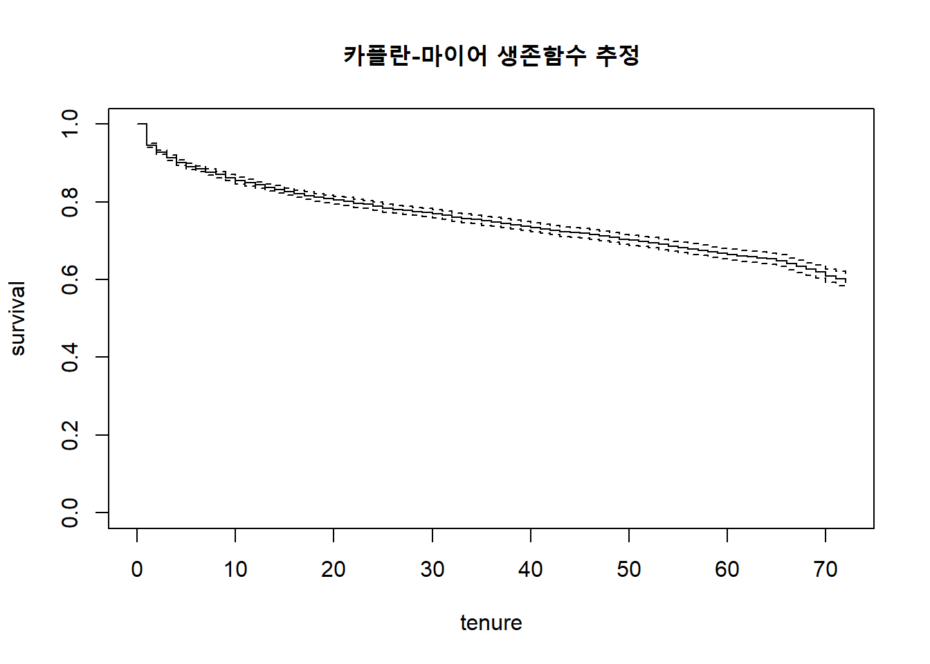

output <- tibble(time=surv.fit$time,
                 surv=surv.fit$surv) %>% 
  mutate(space=time*surv) %>% 
  summarise(avg_life_time=mean(space)) %>%
  pull()


print(output)

[1] 25.68115

생존함수에서 구한 평균이 실제 구독 기간의 평균을 의미하는 것은 아님. 하지만 해당 추정치는 고객 유지 예산 예산 배정의 문제에 도움을 줄 수 있음(Linoff and Berry 2011).

surv.fit <- survfit(Surv(time, status) ~ internet.service,
                    data=churnTel)

Hazard의 경향 확인

time \(t\)에 대한 Hazard는 \[\frac {\text{The number of events at time t}} {\text{population at risk at time t}} \]

(Linoff and Berry 2011).

Kaplan-Meier 적합 시 생성되는 table을 활용하여 데이터로부터 경험적 Hazard ratio를 구할 수 있음.

구독 모델의 경우 초기 진입 이후 프로모션이 끝나면 이탈하는 고객이 있음으로 시간에 따른 Hazard의 모양은 U-자형으로 보임.

tibble(time=surv.fit$time,
       n.event=surv.fit$n.event,
       n.risk=surv.fit$n.risk) %>%
  mutate(hazard.ratio=n.event/n.risk) %>% 
  ggplot() +
  geom_line(aes(x=time, y=hazard.ratio)) +
  ggtitle("72주 기간 동안 hazard ratio의 경향")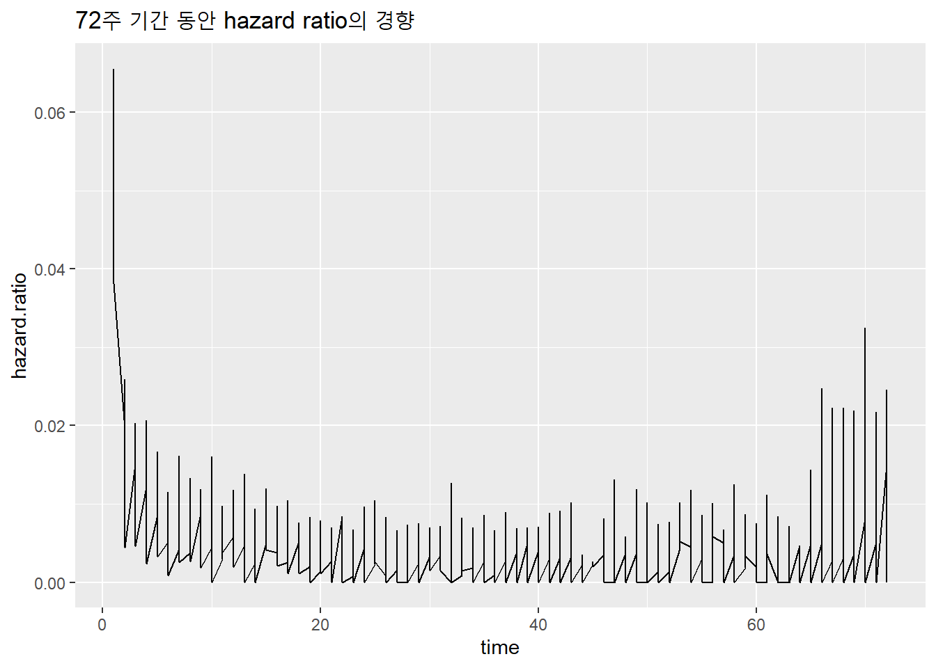

Cox 비례 위험 모형

idx <- churnTel %>% 
  mutate(idx = row_number()) %>% 
  filter(internet.service != "no") %>% 
  filter(phone.service != "no") %>% 
  pull(idx)

data <- churnTel[idx, ] %>% 
  mutate(across(where(is.factor), droplevels)) %>% 
  select(-c(customer.ID, phone.service, total.charge))

N <- nrow(data) * 0.2
test <- sample(nrow(data), N)
train <- setdiff(1:nrow(data), test)

coxph.churn <- 
  coxph(Surv(tenure, churn=="yes") ~ .,
                     data=data,
                     subset=train)

비례위험모형

\[\lambda_{\textbf{x}_i} (t) = \lambda_{0} (t) e^{\beta^t \textbf{x}_i}\]

Cox 비례 위험 모형을 구축함. phone, internet service를 모두 구독하는 고객에 대해서만 Cox 모델 적합을 수행함. (no phone or internet service 고객에 대해서도 모형 적합 시 일부 계수값이 정해지지 않음)

coefficients(summary(coxph.churn))

                                      coef  exp(coef)   se(coef)            z
gendermale                     -0.14000649 0.86935259 0.05668604  -2.46985833
senior.citizen                 -0.06279092 0.93913981 0.06713907  -0.93523658
partnerno                       0.56322692 1.75633091 0.06705128   8.39994266
dependentno                    -0.04698411 0.95410256 0.08255439  -0.56912917
multiple.linesno                0.57683107 1.78038756 0.14661067   3.93444135
internet.servicefiber-optic    -0.04586767 0.95516835 0.66911320  -0.06854994
online.securityno               0.78080968 2.18323928 0.15684596   4.97819434
online.backupno                 0.76636692 2.15193389 0.14736252   5.20055535
device.protectionno             0.41632388 1.51637692 0.14670234   2.83788173
tech.supportno                  0.49446794 1.63962563 0.15606867   3.16827162
streaming.TVno                  0.13869006 1.14876799 0.27639848   0.50177576
streaming.movieno               0.37370181 1.45310378 0.27419150   1.36292267
contract1-year                 -1.45230251 0.23403081 0.10806781 -13.43880738
contract2-year                 -2.81371129 0.05998197 0.20275502 -13.87739423
paperless.billno               -0.18590050 0.83035621 0.06951982  -2.67406465
payment.methodcredit-card      -0.05676702 0.94481417 0.10967605  -0.51758812
payment.methodelectronic-check  0.58746196 1.79941563 0.08558140   6.86436502
payment.methodmail-check        0.46141960 1.58632434 0.11183417   4.12592685
monthly.charge                  0.01759745 1.01775320 0.02667217   0.65976814
                                   Pr(>|z|)
gendermale                     1.351666e-02
senior.citizen                 3.496664e-01
partnerno                      4.466967e-17
dependentno                    5.692685e-01
multiple.linesno               8.339043e-05
internet.servicefiber-optic    9.453479e-01
online.securityno              6.418020e-07
online.backupno                1.986939e-07
device.protectionno            4.541401e-03
tech.supportno                 1.533482e-03
streaming.TVno                 6.158253e-01
streaming.movieno              1.729069e-01
contract1-year                 3.581625e-41
contract2-year                 8.684410e-44
paperless.billno               7.493800e-03
payment.methodcredit-card      6.047457e-01
payment.methodelectronic-check 6.678766e-12
payment.methodmail-check       3.692446e-05
monthly.charge                 5.094026e-01

모형의 평가

\[c = Pr(y_i > y_j | x_i > x_j)\]

모형의 평가지표로 Concordance index(c-index)를 사용할 수 있음. 이는 모든 개체 짝 중 이벤트의 발생이 먼저 일어난 개체가 상대적 위험도 높은 짝의 비율을 계산한 것임(T. Therneau and Atkinson 2023). 수식은 위와 같음.

concordance(coxph.churn)

Call:
concordance.coxph(object = coxph.churn)

n= 3866 
Concordance= 0.8532 se= 0.004359
concordant discordant     tied.x     tied.y    tied.xy 
   2794193     480630         22      40501          4

Cox 비례 위험 모형의 predict는 아래와 같이 5가지의 type을 지원함(T. M. Therneau and Lumley 2015).

\[\hat \lambda_{\textbf{x}_i} (t) = \hat \lambda_{0} (t) e^{\hat \beta^t \textbf{x}_i}\]

lp: the linear predictor \(\hat \beta^t \textbf{x}_i\)
risk: the risk score exp(lp) \(e^{\hat \beta^t \textbf{x}_i}\)
terms: the terms of the linear predictor \(\hat \beta_1 \textbf{x}_1, \cdots, \beta_p \textbf{x}_p\)
expected: the expected number of events given the covariates and follow-up time \(\int^{t}_{0} \hat \lambda_{\textbf{x}_i} (t) dt\)
survival: The survival probability for a subject is equal to exp(-expected) \(\hat S_{\textbf{x}_i} (t) = -\exp (\int^{t}_{0} \hat \lambda_{\textbf{x}_i} (t) dt)\)

모형의 활용

lp: the linear predictor \(\hat \beta^t \textbf{x}_i\)

predict(coxph.churn, data[test, ][1:5, ], type = "lp", , reference="sample")

       792       1483       5275       6401       3608 
-0.5829918  3.8812743 -0.4181787 -1.4452981  1.1453120

X <- subset(model.matrix(churn ~ ., data[test, ])[,2:21], select=-tenure)
new.X <- X - rep(coxph.churn$means, each=nrow(X))
(new.X %*% coef(coxph.churn))[1:5, ]

       792       1483       5275       6401       3608 
-0.5829918  3.8812743 -0.4181787 -1.4452981  1.1453120

risk: the risk score exp(lp) \(e^{\hat \beta^t \textbf{x}_i}\)

predict(coxph.churn, data[test, ][1:5, ], type = "risk", reference="sample")

       792       1483       5275       6401       3608 
 0.5582258 48.4859620  0.6582446  0.2356758  3.1434221

exp((new.X %*% coef(coxph.churn))[1:5, ])

       792       1483       5275       6401       3608 
 0.5582258 48.4859620  0.6582446  0.2356758  3.1434221

terms: the terms of the linear predictor \(\hat \beta_1 \textbf{x}_1, \cdots, \beta_p \textbf{x}_p\)

predict(coxph.churn, data[test, ][1, ], type = "terms", reference="sample")

        gender senior.citizen   partner   dependent multiple.lines
792 -0.1400065              0 0.5632269 -0.04698411              0
    internet.service online.security online.backup device.protection
792                0               0             0                 0
    tech.support streaming.TV streaming.movie  contract paperless.bill
792    0.4944679    0.1386901               0 -1.452303              0
    payment.method monthly.charge
792    -0.05676702    -0.08331659
attr(,"constant")
[1] 1.43656

coef(coxph.churn) * new.X[1, ]

expected: the expected number of events given the covariates and follow-up time \(\int^{t}_{0} \hat \lambda_{\textbf{x}_i} (t) dt\)

predict(coxph.churn, data[test, ][1:5, ], type = "expected", reference="sample")

[1] 0.10601990 0.87958365 0.09528528 0.08211137 0.05702481

survival: The survival probability for a subject is equal to exp(-expected) \(\hat S_{\textbf{x}_i} (t) = -\exp (\int^{t}_{0} \hat \lambda_{\textbf{x}_i} (t) dt)\)

predict(coxph.churn, data[test, ][1:5, ], type = "survival")

[1] 0.8994067 0.4149556 0.9091135 0.9211694 0.9445706

exp(-predict(coxph.churn, data[test, ][1:5, ], type = "expected", reference="sample"))

[1] 0.8994067 0.4149556 0.9091135 0.9211694 0.9445706

상대적 위험도의 값에 따라 고객을 10개의 그룹으로 분류한 후, 그룹 내에서 이탈 고객의 비중을 구하여 모델을 검증할 수 있음(Li 1995).

train 데이터셋의 결과

predicted.risk <- predict(coxph.churn, data[train, ], 
                          type = "risk")

groups <- cut(predicted.risk, breaks = 10)

tibble(groups, 
       predicted.risk, 
       churn=data[train, "churn"]) %>% 
  group_by(groups) %>% 
  count(churn) %>% 
  pivot_wider(names_from=churn, values_from=n) %>% 
  mutate(churn.ratio=round(yes/(yes+no)*100,1))

# A tibble: 10 × 4
# Groups:   groups [10]
   groups           yes    no churn.ratio
   <fct>          <int> <int>       <dbl>
 1 (-0.0469,9.06]   288  1669        14.7
 2 (9.06,18.1]      236   363        39.4
 3 (18.1,27.1]      232   223        51  
 4 (27.1,36.1]      144   137        51.2
 5 (36.1,45.1]      152    92        62.3
 6 (45.1,54.1]       77    49        61.1
 7 (54.1,63.2]       44    26        62.9
 8 (63.2,72.2]       48    23        67.6
 9 (72.2,81.2]       26     9        74.3
10 (81.2,90.3]       20     8        71.4

test 데이터셋의 결과

predicted.risk <- predict(coxph.churn, data[test, ], type = "risk")

groups <- cut(predicted.risk, breaks = 10)
tibble(groups, predicted.risk, churn=data[test, "churn"]) %>% 
  group_by(groups) %>% 
  count(churn) %>% 
  pivot_wider(names_from=churn, values_from=n) %>% 
  mutate(churn.ratio=round(yes/(yes+no)*100,1))

# A tibble: 10 × 4
# Groups:   groups [10]
   groups           yes    no churn.ratio
   <fct>          <int> <int>       <dbl>
 1 (-0.0403,8.32]    65   428        13.2
 2 (8.32,16.6]       64    74        46.4
 3 (16.6,24.9]       54    62        46.6
 4 (24.9,33.2]       36    33        52.2
 5 (33.2,41.4]       39    17        69.6
 6 (41.4,49.7]       24    16        60  
 7 (49.7,58]         10     6        62.5
 8 (58,66.3]          6     3        66.7
 9 (66.3,74.6]       13     8        61.9
10 (74.6,82.9]        8    NA        NA

참고문헌

James, Gareth, Daniela Witten, Trevor Hastie, Robert Tibshirani, et al. 2013. An Introduction to Statistical Learning. Vol. 112. Springer.

Li, Shaomin. 1995. “Survival Analysis.” Marketing Research 7 (4): 16.

Linoff, Gordon S, and Michael JA Berry. 2011. Data Mining Techniques: For Marketing, Sales, and Customer Relationship Management. John Wiley & Sons.

Mohammadi, Reza, and Kevin Burke. 2023. Liver: "Eating the Liver of Data Science". https://CRAN.R-project.org/package=liver.

Therneau, Terry M, and Thomas Lumley. 2015. “Package ‘Survival’.” R Top Doc 128 (10): 28–33.

Therneau, Terry, and Elizabeth Atkinson. 2023. “1 the Concordance Statistic.”

서영정. 2023. “머신러닝 기반 생존분석기법을 활용한 고객 이탈 예측 기술.” Journal of Digital Contents Society 24 (8): 1871–80.

허명회. 2023. “응용데이터분석방법론 4. 생존분석 강의노트.”