!pip install prophet plotly -Uqq시계열 분석 라이브러리인 Prophet을 사용합니다. 아래와 같은 장점이 있습니다.
- 빠른 모델 구축 및 성능 평가
- 쉬운 하이퍼파라미터 조정
import pandas as pd
from prophet import Prophet
데이터 확인
train = pd.read_csv('train.csv')pandas로 train을 불러옵니다. 이 대회는 train, test가 따로 주어진 것이 아닙니다.
train.head()| 일시 | 광진구 | 동대문구 | 성동구 | 중랑구 | |
|---|---|---|---|---|---|
| 0 | 20180101 | 0.592 | 0.368 | 0.580 | 0.162 |
| 1 | 20180102 | 0.840 | 0.614 | 1.034 | 0.260 |
| 2 | 20180103 | 0.828 | 0.576 | 0.952 | 0.288 |
| 3 | 20180104 | 0.792 | 0.542 | 0.914 | 0.292 |
| 4 | 20180105 | 0.818 | 0.602 | 0.994 | 0.308 |
print(f'{len(train)} 개의 행') 1461 개의 행train['일시'] = pd.to_datetime(train['일시'], format='%Y%m%d')train.describe(datetime_is_numeric=True)| 일시 | 광진구 | 동대문구 | 성동구 | 중랑구 | |
|---|---|---|---|---|---|
| count | 1461 | 1461.000000 | 1461.000000 | 1461.000000 | 1461.000000 |
| mean | 2020-01-01 00:00:00 | 6.209194 | 4.233670 | 5.182951 | 3.138747 |
| min | 2018-01-01 00:00:00 | 0.000000 | 0.000000 | 0.000000 | 0.000000 |
| 25% | 2019-01-01 00:00:00 | 3.256000 | 2.068000 | 2.676000 | 1.456000 |
| 50% | 2020-01-01 00:00:00 | 5.740000 | 3.588000 | 4.850000 | 2.596000 |
| 75% | 2020-12-31 00:00:00 | 9.444000 | 6.212000 | 7.704000 | 4.768000 |
| max | 2021-12-31 00:00:00 | 15.184000 | 11.708000 | 13.366000 | 8.028000 |
| std | NaN | 3.531408 | 2.695602 | 2.937556 | 2.046930 |
initial = ['g', 'd', 's', 'j']district = list(zip(initial, train.columns.values[1:]))district[('g', '광진구'), ('d', '동대문구'), ('s', '성동구'), ('j', '중랑구')]하나의 구만 뜯어서 실험해본 뒤 다른 행정구로 넓히어 적용하겠습니다.
train_g = train.loc[:, ['일시', '광진구']]train_g.columns = ['ds', 'y']val_g = train_g[train_g.ds >= '2021-01-01']
train_g = train_g[train_g.ds < '2021-01-01']train_g| ds | y | |
|---|---|---|
| 0 | 2018-01-01 | 0.592 |
| 1 | 2018-01-02 | 0.840 |
| 2 | 2018-01-03 | 0.828 |
| 3 | 2018-01-04 | 0.792 |
| 4 | 2018-01-05 | 0.818 |
| ... | ... | ... |
| 1091 | 2020-12-27 | 3.528 |
| 1092 | 2020-12-28 | 4.542 |
| 1093 | 2020-12-29 | 3.694 |
| 1094 | 2020-12-30 | 2.366 |
| 1095 | 2020-12-31 | 2.366 |
1096 rows × 2 columns
초기 모델 생성
m = Prophet()add_seasonality는 모델에 계절성 요소 추가를 위해 사용합니다.
m.add_seasonality(name='yearly', period=365.25, fourier_order=10, prior_scale=10, mode='additive')
m.add_seasonality(name='monthly', period=30.5, fourier_order=7, prior_scale=10, mode='additive')
m.add_seasonality(name='weekly', period=7, fourier_order=3, prior_scale=10, mode='additive')
<prophet.forecaster.Prophet at 0x7f90d4e40e20>m.fit(train_g)07:28:37 - cmdstanpy - INFO - Chain [1] start processing
07:28:37 - cmdstanpy - INFO - Chain [1] done processing<prophet.forecaster.Prophet at 0x7f90d4e40e20>future = m.make_future_dataframe(periods=365)
future.tail()| ds | |
|---|---|
| 1456 | 2021-12-27 |
| 1457 | 2021-12-28 |
| 1458 | 2021-12-29 |
| 1459 | 2021-12-30 |
| 1460 | 2021-12-31 |
forecast = m.predict(future)forecast.head()| ds | trend | yhat_lower | yhat_upper | trend_lower | trend_upper | additive_terms | additive_terms_lower | additive_terms_upper | monthly | ... | weekly | weekly_lower | weekly_upper | yearly | yearly_lower | yearly_upper | multiplicative_terms | multiplicative_terms_lower | multiplicative_terms_upper | yhat | |
|---|---|---|---|---|---|---|---|---|---|---|---|---|---|---|---|---|---|---|---|---|---|
| 0 | 2018-01-01 | 2.658666 | -2.875560 | 1.674994 | 2.658666 | 2.658666 | -3.225742 | -3.225742 | -3.225742 | 0.252489 | ... | -0.035986 | -0.035986 | -0.035986 | -3.442245 | -3.442245 | -3.442245 | 0.0 | 0.0 | 0.0 | -0.567076 |
| 1 | 2018-01-02 | 2.661896 | -2.491145 | 1.998054 | 2.661896 | 2.661896 | -2.957412 | -2.957412 | -2.957412 | 0.278704 | ... | 0.159656 | 0.159656 | 0.159656 | -3.395773 | -3.395773 | -3.395773 | 0.0 | 0.0 | 0.0 | -0.295517 |
| 2 | 2018-01-03 | 2.665125 | -3.017387 | 1.560996 | 2.665125 | 2.665125 | -3.360643 | -3.360643 | -3.360643 | 0.013977 | ... | -0.029910 | -0.029910 | -0.029910 | -3.344710 | -3.344710 | -3.344710 | 0.0 | 0.0 | 0.0 | -0.695518 |
| 3 | 2018-01-04 | 2.668354 | -3.190014 | 1.344889 | 2.668354 | 2.668354 | -3.594391 | -3.594391 | -3.594391 | -0.279672 | ... | -0.024221 | -0.024221 | -0.024221 | -3.290498 | -3.290498 | -3.290498 | 0.0 | 0.0 | 0.0 | -0.926037 |
| 4 | 2018-01-05 | 2.671583 | -2.805003 | 1.613210 | 2.671583 | 2.671583 | -3.467301 | -3.467301 | -3.467301 | -0.360179 | ... | 0.127509 | 0.127509 | 0.127509 | -3.234630 | -3.234630 | -3.234630 | 0.0 | 0.0 | 0.0 | -0.795718 |
5 rows × 22 columns
forecast.loc[:, ['ds', 'yhat']]| ds | yhat | |
|---|---|---|
| 0 | 2018-01-01 | -0.567076 |
| 1 | 2018-01-02 | -0.295517 |
| 2 | 2018-01-03 | -0.695518 |
| 3 | 2018-01-04 | -0.926037 |
| 4 | 2018-01-05 | -0.795718 |
| ... | ... | ... |
| 1456 | 2021-12-27 | 2.228512 |
| 1457 | 2021-12-28 | 2.356364 |
| 1458 | 2021-12-29 | 2.182632 |
| 1459 | 2021-12-30 | 2.369206 |
| 1460 | 2021-12-31 | 2.674375 |
1461 rows × 2 columns
예측값이 0보다 작을 수는 없으니 0보다 작은 경우 0으로 바꾸어 줍니다.
import numpy as npforecast.yhat = np.where(forecast.yhat < 0, 0, forecast.yhat)val_g| ds | y | |
|---|---|---|
| 1096 | 2021-01-01 | 2.070 |
| 1097 | 2021-01-02 | 2.062 |
| 1098 | 2021-01-03 | 1.918 |
| 1099 | 2021-01-04 | 3.238 |
| 1100 | 2021-01-05 | 2.864 |
| ... | ... | ... |
| 1456 | 2021-12-27 | 3.830 |
| 1457 | 2021-12-28 | 4.510 |
| 1458 | 2021-12-29 | 4.490 |
| 1459 | 2021-12-30 | 4.444 |
| 1460 | 2021-12-31 | 3.616 |
365 rows × 2 columns
train_g| ds | y | |
|---|---|---|
| 0 | 2018-01-01 | 0.592 |
| 1 | 2018-01-02 | 0.840 |
| 2 | 2018-01-03 | 0.828 |
| 3 | 2018-01-04 | 0.792 |
| 4 | 2018-01-05 | 0.818 |
| ... | ... | ... |
| 1091 | 2020-12-27 | 3.528 |
| 1092 | 2020-12-28 | 4.542 |
| 1093 | 2020-12-29 | 3.694 |
| 1094 | 2020-12-30 | 2.366 |
| 1095 | 2020-12-31 | 2.366 |
1096 rows × 2 columns
import matplotlib.pyplot as pltt = (forecast
.loc[:, ['ds', 'yhat']]
.merge(train_g)
)plt.scatter(t['ds'], t['y'], s=10)
plt.scatter(t['ds'], t['yhat'], s=10)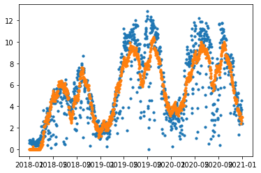
모델은 train_g(2018-01~2021-12) 기간을 위와 같이 훈련했습니다.
t = (forecast[forecast.ds >= '2021-01-01']
.loc[:, ['ds', 'yhat']]
.merge(val_g)
.assign(se = lambda x: (x.yhat - x.y)**2)
)plt.scatter(t['ds'], t['y'], s=10)
plt.scatter(t['ds'], t['yhat'], s=10)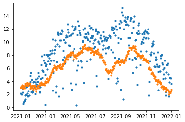
그 결과로 val_g를 위와 같이 예측했습니다.
실제값의 변동은 굉장히 크지만, Prophet은 부드러운 곡선으로 미래를 예측했습니다.
t['se'].mean()11.198355303365641모델 조정
1천명 단위이니 하루 평균 1만명 정도의 차이가 납니다..!
왜 이런 결과가 나왔을까요? - 따릉이는 비 온 날과 오지 않은 날의 인원이 확연히 다릅니다. 비 온 날의 값이 비 오지 않은 날의 인원까지도 낮춘 것으로 보입니다. 예시로, 2019, 2020년 장마 기간에 따라 따릉이 이용이 줄어들었는데, 2021년에는 장마가 늦춰진다면 예측이 실패할 것입니다.
차이를 줄이기 위해 예측값에서 일정 수를 더해주면 되지 않을까요? 아래와 같이 말입니다.
t = (forecast[forecast.ds >= '2021-01-01']
.loc[:, ['ds', 'yhat']]
.merge(val_g)
.assign(yhat = lambda x: x.yhat + 3) # 3을 더함
.assign(se = lambda x: (x.yhat - x.y)**2)
)plt.scatter(t['ds'], t['y'], s=10)
plt.scatter(t['ds'], t['yhat'], s=10)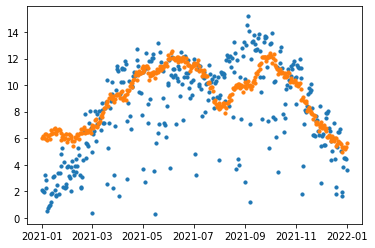
t['se'].mean()8.005238250656378겨울은 비가 올 일이 적으니 예측값을 보정하지 않고 여름은 비 오는 날이 많으니 예측값에서 더 많이 더해볼까요?
month_winter = [1]
month_summer = [8]def consider_month(x):
if x.ds.month in month_winter:
return x.yhat
elif x.ds.month in month_summer:
return x.yhat + 6
else:
return x.yhat + 3t = (forecast[forecast.ds >= '2021-01-01']
.loc[:, ['ds', 'yhat']]
.merge(val_g)
)
t['yhat'] = t.apply(lambda x: consider_month(x), axis=1)
t['se'] = (t.yhat - t.y)**2plt.scatter(t['ds'], t['y'], s=10)
plt.scatter(t['ds'], t['yhat'], s=10)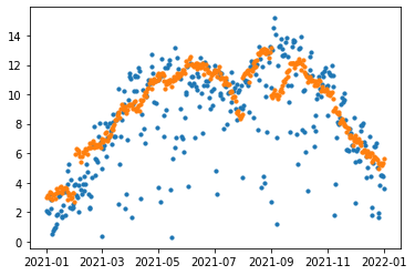
t['se'].mean()7.274777463700824지금까지 하나의 행정구에 대해 보았던 내용을 함수를 만들어 반복시키겠습니다.
- 구별 칼럼마다,
- 일시와 구별 데이터프레임을 생성합니다.
- ‘2021-01-01’ 이후 데이터를 validation, ‘2021-01-01’ 이전 데이터를 train으로 구분합니다.
- 모델을 생성합니다.
- validation에 대한 예측값을 생성하고, 실제값과 비교하는 플롯을 그립니다.
- MAE 값을 보여줍니다.
def train_test_split(train_d, date :str):
train_d.columns = ['ds', 'y']
val_d = train_d[train_d.ds >= date]
train_d = train_d[train_d.ds < date]
return train_d, val_ddef make_model():
m = Prophet()
m.add_seasonality(name='yearly', period=365.25, fourier_order=10, prior_scale=10, mode='additive')
m.add_seasonality(name='monthly', period=30.5, fourier_order=5, prior_scale=10, mode='additive')
m.add_seasonality(name='weekly', period=7, fourier_order=3, prior_scale=10, mode='additive')
return mfor i, (_, d) in enumerate(district):
print(i, d)0 광진구
1 동대문구
2 성동구
3 중랑구def mae():
t = (forecast[forecast.ds >= '2021-01-01']
.loc[:, ['ds', 'yhat']]
.merge(val_d)
)
t['yhat'] = t.apply(lambda x: consider_month(x), axis=1)
t['se'] = np.abs(t.yhat - t.y)
return t['se'].mean()def plot_forecast():
t = (forecast
    .loc[:, ['ds', 'yhat']]
    .merge(train_g)
)
t['yhat'] = t.apply(lambda x: consider_month(x), axis=1)
t['se'] = np.abs(t.yhat - t.y)
ax.scatter(t['ds'], t['y'], s=10)
ax.scatter(t['ds'], t['yhat'], s=10)def sub_predict():
t = (forecast
.loc[forecast.ds >= '2022-01-01', ['ds', 'yhat']]
)
t['yhat'] = t.apply(lambda x: consider_month(x), axis=1)
sample_submission[d] = (t
.loc[:, ['yhat']]['yhat']
.to_numpy()
)제출
sample_submission = pd.read_csv('sample_submission.csv')fig = plt.figure(figsize=(12, 6))
for i, (_, d) in enumerate(district):
ax = fig.add_subplot(2,2,i+1)
train_d = train.loc[:, ['일시', d]]
train_d, val_d = train_test_split(train_d, '2021-01-01')
m = make_model()
m.fit(train_d)
future = m.make_future_dataframe(periods=365*2-31)
forecast = m.predict(future)
forecast.yhat = np.where(forecast.yhat < 0, 0, forecast.yhat)
metric = mae()
print(f'{d}: MAE {metric}')
plot_forecast()
sub_predict()07:28:39 - cmdstanpy - INFO - Chain [1] start processing
07:28:39 - cmdstanpy - INFO - Chain [1] done processing
07:28:40 - cmdstanpy - INFO - Chain [1] start processing광진구: MAE 1.872618177797537307:28:40 - cmdstanpy - INFO - Chain [1] done processing
07:28:41 - cmdstanpy - INFO - Chain [1] start processing동대문구: MAE 2.148040836722335407:28:41 - cmdstanpy - INFO - Chain [1] done processing
07:28:43 - cmdstanpy - INFO - Chain [1] start processing성동구: MAE 2.65069455823116207:28:43 - cmdstanpy - INFO - Chain [1] done processing중랑구: MAE 3.0494228125293197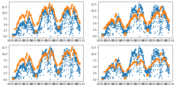
sample_submission| 일시 | 광진구 | 동대문구 | 성동구 | 중랑구 | |
|---|---|---|---|---|---|
| 0 | 20220101 | 2.517673 | 3.804060 | 3.729617 | 3.678316 |
| 1 | 20220102 | 2.165276 | 3.467720 | 3.546800 | 3.423660 |
| 2 | 20220103 | 2.582113 | 4.115750 | 4.111609 | 3.673531 |
| 3 | 20220104 | 2.909643 | 4.426972 | 4.424393 | 3.935403 |
| 4 | 20220105 | 2.741750 | 4.275806 | 4.176622 | 3.881529 |
| ... | ... | ... | ... | ... | ... |
| 329 | 20221126 | 6.629785 | 8.867939 | 8.395034 | 8.393789 |
| 330 | 20221127 | 6.050292 | 8.437032 | 8.061970 | 8.048558 |
| 331 | 20221128 | 6.292194 | 9.013169 | 8.508141 | 8.218626 |
| 332 | 20221129 | 6.537858 | 9.272077 | 8.749229 | 8.411412 |
| 333 | 20221130 | 6.385127 | 9.077534 | 8.471963 | 8.299933 |
334 rows × 5 columns
sample_submission.to_csv('sub.csv', index=False)